Damped Harmonic Motion

Have you ever thought about making a damped pendulum in Grasshopper? I have no idea why, but I did. I just decided to transfer a Python snippet I found online into a Grasshopper definition. Here, the Initial Angle (Radians) Number slider sets the initial angle to any value from 0 to Pi. The letter G represents the acceleration due to gravity (approximately 9.81 m/s²). This is the primary force pulling the pendulum downward. As you know, pendulums wouldn’t swing without gravity. And L is simply the length of the pendulum. Let’s go:

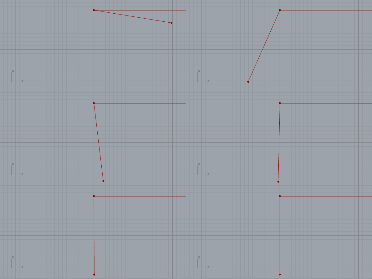
Simple Harmonic Motion

According to Wikipedia, if a body moves around a circle, its motion is a simple harmonic motion with an amplitude of r and an angular frequency (angular velocity) of omega. While I didn’t entirely know where the Sqrt(g/l) in my code came from, that encyclopedia article also points out a 2pi multiplier in that formula. An interesting takeaway here is that the period of oscillation is independent of the pendulum’s mass but depends on the acceleration due to gravity. The same formula is also mentioned under Newton’s second law and here.

Exponential Damping

The next section of the Grasshopper definition serves as the core engine calculating the pendulum’s angle at any given moment (t). Naturally, we need some damping here. We handle this damping using an exponential function, which relies on a special constant called e (Euler’s number). We raise e to the power of x. Here, we use t for time and d for the damping (or friction) coefficient. When time t = 0 (since time hasn’t started ticking yet), e to the power of zero equals 1, meaning no damping occurs at first. As time goes on, the exponent increases along with the damping coefficient, and the result rapidly approaches zero. That was my best attempt at understanding it anyway. This value was tied to time as our damping multiplier. We then multiply this by the initial angle (in radians) and the time-dependent Simple Harmonic Motion (see the previous section).

Pendulum Position

The value obtained by multiplying these three components is the pendulum’s angle at time t. Now, all we have to do is use this angle and the length (L) with Grasshopper’s “Point Polar” component to position the tip of the pendulum. For aesthetic reasons, we rotated the angle by 90 degrees so the pendulum points downward on the screen. I know, this part wasn’t elegant at all, but it got the job done. In the end, we managed to build our damped pendulum simulator in Grasshopper.

What I found interesting throughout this process was how I kept trying to investigate why things were the way they were while attempting to adapt a snippet of code into Grasshopper. Thanks to this code, I realized that certain things can be done without using loops like Anemone. Even though the formulas are laid out clearly in the Wikipedia links I shared with you, I couldn’t find an answer to the “Why?” question. Sometimes a formula can be deceptively simple. As a designer, understanding and modeling this is fun up to a point, but sometimes I catch myself thinking, “I wish I had studied more physics and math.” Today, we really ought to question the fundamental physics and math education of architects who call themselves computational designers (myself included). Sure, we’re good at applying formulas, coding, and visualizing the results, and assuming that we understand everything. But if someone asked me to develop this code entirely from scratch without any outside help, I couldn’t have done it. All I can do is let the ignorance I feel in situations like this drive me to experiment even more.