Curve Continuity

Continuity in piecewise Bézier curves was one of the important topics of our first-year architecture geometry course. Here, I will briefly summarize what this course attempts to convey. Since there are many ways to define it, I have summarized them below and tried to indicate how each is perceived visually.

C0: Position Continuity

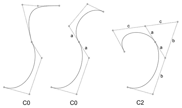
This refers simply to the end-to-end connection of two Bézier curve segments; there are no gaps between the curves. The endpoint of the first curve is on the starting point of the second curve. The curve is geometrically continuous, but a sharp break (corner/kink) may exist at the joint. Tangents and curvature are not compatible.

C1: Tangent Continuity

Beyond positional continuity, this ensures that the tangent vectors at the junction point are also equal in direction and magnitude. Thus, the first derivatives are continuous. The first derivative vector at the end of the first curve equals the first derivative vector at the start of the second curve. The control point preceding the joint, the joint itself, and the subsequent control point lie completely on the same straight line (collinear), and the distances between them are equal. The visual result is a smooth transition. However, because curvature continuity is not yet established, a sudden change in the radius or intensity of the curvature (acceleration/jerk) can be observed. If you turn on the control points of both curves and look at the segments of the joining control polygon, we can say that C1 exists between these two curves if they lie on the same line and are of equal length.

C2: Curvature Continuity

C2 (curvature) continuity of two Bézier curves requires equality of the second derivatives. At the junction point of the curves, not only the tangent vectors, but also the curvatures are equal and connected smoothly. As seen in the visual, a 1:1 ratio is established between the control points at the junction points to form an “A-frame” over the apex. These ratios mathematically guarantee the continuity of the second derivatives (curvature continuity). The knot or parameter intervals k, k+1, and k+2 ensure a smooth transition between two neighboring Bézier segments. You can use whichever of these definitions you prefer. The one that interests me the most, of course, is the visual and geometric one. That is, not only do the control polygon segments tangent to both ends need to be in the same direction and of equal length, but the segments of the A-Frames on top of these segments must also be of equal length. What does this mean?

The Exercise

This must be the most fun exercise of the course. If this is the most fun part of the course, imagine the rest :) How can we draw a C2 continuous curve for any given curve? I tried to show this step by step below. To geometrically construct C2 continuity using the A-frame method (without using commands), the line passing through the last two control points of the existing curve is extended beyond the junction point, and equal 1:1 distances are marked along this axis to determine the tangent control point (C1). Then, the top apex control point is placed over these points to form a triangle (A-frame), creating a visually flawless curvature transition without requiring any commands or formulas. The first three control points of the second curve are now ready in our hand. We can place the fourth and final control point wherever we want. The resulting 3rd-degree Bézier curve will have C2 continuity with the first curve.

Rhino Tools

In Rhino (tested in Rhino 8), commands that establish continuity include MatchCrv, BlendCrv, FilletCrv, and ChamferCrv. Their counterparts for surfaces can be observed in MatchSrf, BlendSrf, NetworkSrf, and Sweep2. Analysis tools related to continuity include GCon (Geometric Continuity) and CurvatureGraph. CurvatureGraph opens a display called a curvature comb. In C1, there is a jump in the comb’s length; in C2, the comb is continuous but has a slope break; in C3, the comb also looks smooth. Additionally, Zebra, EMap, and CurvatureAnalysis (for surfaces) can be mentioned. ShowCP / PointsOn, Rebuild, ChangeDegree, and InsertKnot can be used to display the control point layout and control the degree. I tested these in Rhino 8, and there may be new features in the newly released version 9.