Koch Snowflake Fractal

by Tuğrul Yazar | April 12, 2023 20:21

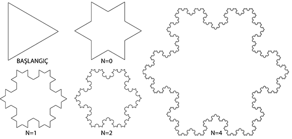
This is an implementation of the famous Koch Snowflake Fractal[2] in Grasshopper[3]. We will be using the Anemone add-on[4] to handle the iterations. In this fractal, we start from an equilateral triangle. Then, we form new equilateral triangles, one-third of the side. So that each repetition protrudes in the middle of all the sides. In summary;
1: Take a closed polygon and divide it into parts and divide each side into three equal parts,
2: Modify the middle piece from the resulting three pieces to form a new pair of equilateral edges,
3: Rejoin the modified shape and return to Step 1.

The Preparation for Koch Snowflake Fractal

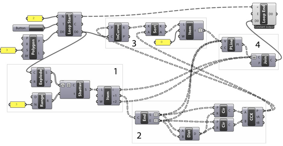
Now let’s follow the Grasshopper application step by step. We start Koch Snowflake Fractal by creating a triangle and feeding it to Loop Start, the startup component of Anemone. In the first step, we’ll start with a large triangle. It will then transform into the star or snowflake-shaped closed polygon you see in the figure. In part 1 of the diagram, we explode the incoming closed polygon to its edges. Then, we divide each of these sides into three equal parts.

When we connect a Panel to the output of the Shatter component, what we will see is a data tree of edges grouped in threes. In the design of the fractal, we delete the middle part of each edge. Then, we create two new equilateral edges in their place. To do this, the data tree we obtained from Shatter is decomposed into its elements with the help of the List Item (Item) component. In this component, the default value of i is 0, that is, the zero index element of the incoming list. When we connect a data tree consisting of three-element data lists to this component, the output i+1 will represent the 1-index element of each data list, which is the middle part that we want to delete and replace.

A Little Euclidean Construction

In the second part of the Koch Snowflake Fractal diagram, we place the two sides of a new equilateral triangle in the middle part. There are several ways to do this, but the most precise is to use Euclidean constructions, the compass method. After we obtained the two ends (start and end points) with the End Points (End) component, we place circles on these two endpoints. If the radius of these circles is exactly the distance between the two points, the intersection point we will obtain will define a new equilateral triangle there. The circles placed at both ends of the middle segment are drawn separately because after a step we will intersect these circles to obtain the vertex of the new triangle. With the help of the Curve I Curve (CCX) intersection component, we intersect the circles. As a result of this process, we obtain two alternatives.

In the next chapter, chapter three, we determine which of these two points should be taken and which should be ignored. In the design of the fractal, the newly produced edges always open outward from the shape, and no edges are formed inwardly. We use a component called Point In Curve (InCurve) to describe this situation to Grasshopper. This component reports whether a point is inside a given curve. Our fractal yields a new closed polygon at the end of each step. One of the two points we have just found by intersecting the circles always comes out of the closed polygon one step earlier, and the other is inside. Taking advantage of this geometric situation, the Point In Curve (InCurve) component will tell us which of these points is inward and which is outward.

Some Tricks of Dataflow

The R output of the component consists of the numbers 0 and 2. The number 0 indicates that the point with that address is outside the curve. The number 2 indicates that that point is inside the curve. Here we understand that we need points coded with 0. So how can we use this encoding? We can use several different methods to extract the desired points from the output of the Curve I Curve (CCX) component. In the example, we do this by making a simple Sort List (Sort). We know that the Sort List component could not only sort numbers from smallest to largest but also arrange in parallel any other list with the same addressing that we would give in parallel to this array.

Using this feature, we connect the output of Point In Curve (InCurve), consisting of 0 and 2, to the K input of the Sort List (Sort), and we ensure that each data list is arranged in order from smallest to largest. This sequence will make the result code 0 the first element of the data lists. What we really need is to arrange the two-point data lists we have in parallel with this sequence. When this list, which we have connected to the A input of the Sort List component, comes back to us in a rearranged form from the A output, it means that our points outside the curve are coded with 0. All we have to do is to pull the data with index 0 with the help of a List Item (Item) component.

Final Step of the Iteration

In the fourth and final part of the Koch Snowflake Fractal diagram, we collect the new version of the curve. We need to get a new polygon at the end of each step. So we can send it to the beginning of the next step. We have to redraw the middle section of each segment. For this, we need to enter the points in the Polyline (Pline) component in the correct order (by pressing shift). Our first point is the starting point of the middle segment that we are going to delete. The second point is the point where we just got the final version.

Finally, we must connect the end point of the middle segment. When we do this, we make the desired drawing instead of the deleted middle segment. Finally, with these new polylines, we combine the two existing segments to construct the entire shape. Using the Join Curves (Join) component, we combine the first segment of the exploding edge, then the new two-sided polyline that we just drew, and finally the segment at the other end of the edge.

Finishing the Koch Snowflake Fractal

After this point, we return to the beginning with the Loop End. We repeat the whole process using the new shape. We changed the Constant&Record mode in the right-click menu of the Loop End component to Constant Output this time. Thanks to this change, Anemone will only show the result in the last iteration. Normally drawing such a shape without Anemone would be a much more challenging process. It would require a complex and large diagram. Because we would need to repeatedly copy all the diagram elements for each step. Nor would we have the flexibility to change the number of steps.

If you change some parameters while playing with Anemone, click the Button connected to the T input. So Grasshopper runs the loop from the beginning. Applying repetition 4 times to this application requires combining and breaking 2304 edges. This number increases to 9216 edges in step 5. Then, 36864 edges in step 6, and 147456 edges in step 7. So we do not recommend you try more than 3-4 steps in order not to crash your computer.

You can re-build the definition by looking at the image above and the explanation. However, if you liked this content and want to download the Grasshopper file; would you consider being my Patreon? Here is the link to my Patreon page[5] including the working Grasshopper file for the Koch Snowflake Fractal.

Source URL: https://www.designcoding.net/koch-snowflake-fractal/

---