Fourier Transform

by Tuğrul Yazar | November 14, 2022 14:06

The first trial of Discrete Fourier Transform in Grasshopper and Python. The technique is used to decompose a function into its frequency components. There are many uses for this technique in physics and engineering. However, the interesting and intuitive part of this mathematical technique is the way of its visualization and the potential mathematical “magic” it produces. I found several examples on the internet of this beautiful visualization such as Coding Train[1] and 3Blue1Brown[2] and Mathologer[3]. They all explain the concept and method from different starting points, and all are very good explanations.

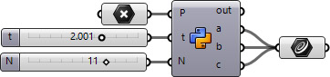
Below is the Grasshopper code that includes a Python component to do this animation. It draws the circles and the resulting wave. This is only the beginning of more complex things. You can play with the N input to change the number of circles and see the resulting wave. The t input helps to change the rotation of the circles, enabling the animation seen above. This is a work in progress, testing the basics of the technique only. Of course, the more interesting study would be reversing this process and determining the circle combinations of a given wave, which is the real function of this mathematical method.

import rhinoscriptsyntax as rs
import math

a = []
b = []
c = []
dt = math.pi / 200
t =  - 2 * t * math.pi

# Circles
x = P[0]
y = P[1]
for i in range(N):
    prevx = x
    prevy = y
    n = i * 2 + 1
    radius = 4 / (n * math.pi)
    x += radius * math.cos(n * t)
    y += radius * math.sin(n * t)
    a.append(rs.AddCircle([prevx,prevy,0], radius))
    a.append(rs.AddCircle([x,y,0], 0.02))
    b.append(rs.AddLine([x,y,0],[prevx,prevy,0]))

# Wave
t_wave = 2 * math.pi
wave_pts = []
while t_wave > 0:
    wave_y = P[1]
    for i in range(N):
        n = i * 2 + 1
        radius = 4 / (n * math.pi)
        wave_y += radius * math.sin(n * (t + (t_wave)))
    temp_pt = [3.6 + (t_wave / 2), wave_y, 0]
    wave_pts.append(temp_pt)
    t_wave -= dt

# Output
c.append(rs.AddInterpCurve(wave_pts))
b.append(rs.AddLine([x,y,0],[3.6, y, 0]))

Above is the Fourier Transform code I wrote in the Python[4] component. It should work in Rhino 6 and 7 without problems. I will leave the detailed explanation of the code to another post. However, You can rebuild the component by copying the code above. However, if you liked this content and want to download the Grasshopper file; would you consider being my Patreon? Here is the link to my Patreon page[5] including the working Grasshopper file for the Fourier Transform.

Source URL: https://www.designcoding.net/fourier-transform/